Published On Apr 24, 2024
In one word, blurry.
In this simulation, a light source moving at about 1.2 times the speed of light is observed through a gradient index lens. This is of course not possible in our relativistic universe, though it can be done with sound waves or water waves. As a result of its high speed, the source creates a shock wave, and that is what is observed in the focal plane shown on the right.
The refractive index n(r) depends on the distance r to the horizontal symmetry axis of the lens in a quadratic way, like n(r) = n0 - a*r², with n0 = 1.25 and a = 0.4375, making the refractive index smaller than 1 at the outer boundary of the lens, where r = 1. In order to visualize the refractive index as well, the luminosity of the background depends on the refractive index.
The videos are inspired by Huygens Optics' recent short • Gradient Index Lens Explained showing the principle of a gradient index lens.
Lenses focus incoming rays of light by delaying them more near the center of the lens than at its periphery. This is often done with a material of constant index of refraction, by making the lens thicker near the center, as shown for instance in the simulation • A circular lens, in higher resolution . However, one can also build lenses of constant thickness, by making the index of refraction of their material depend on the location in the lens. In this simulation, the index decreases like the square of the distance to the center (that is, it is of the form n0 - a*r², where r is the distance to the axis of symmetry). This results in the incoming waves being focused at two points in the (estimated) focal plane, marked by a vertical line. The plot to the right shows a time-averaged value of the field along that plane.
This video has two parts, showing the same evolution with two different color gradients:
Wave height: 0:00
Averaged wave energy: 1:31
In the first part, the color hue depends on the height of the wave. In the second part, it depends on the energy of the wave, averaged over a sliding time window.
There are absorbing boundary conditions on the borders of the simulated rectangle. The display at the right shows the signal along the focal plane, which is indicated by a vertical line.
Render time: 43 minutes 52 seconds
Compression: crf 23
Color scheme: Part 1 - Twilight by Bastian Bechtold
https://github.com/bastibe/twilight
Part 2 - Plasma by Nathaniel J. Smith and Stefan van der Walt
https://github.com/BIDS/colormap
Music: "I Don't Remmber I Don't Recall" by the 129ers
See also https://images.math.cnrs.fr/Des-ondes... for more explanations (in French) on a few previous simulations of wave equations.
The simulation solves the wave equation by discretization. The algorithm is adapted from the paper https://hplgit.github.io/fdm-book/doc...
C code: https://github.com/nilsberglund-orlea...
https://www.idpoisson.fr/berglund/sof...
Many thanks to Marco Mancini and Julian Kauth for helping me to accelerate my code!
#wave #lens #gradient_index